As I’m writing this, Dror Helper blogged about using a poor man’s performance profiler. This profiling technique is useful when the tools are lacking, and we need to measure a performance of method(s) within our code. This information is usually logged, and after a run we’re left with a huge file containing hundreds (and sometimes thousands of lines). How do we make sense of this mess? How do we filter out and understand the relevant performance information?
As it happens, Microsoft Excel is a great tool to assist with this task! Excel is this part of Microsoft Office, which everyone has, but very few know how to use. I was watching as a colleague of mine, Doron, worked his magic with Excel, and now I’d like to share this information with the rest of the class:
Note: I used Excel 2010 to perform this. I believe that this is possible with earlier versions, but I can’t tell for sure.
We start by opening the log file, selecting all text, and pasting it into a new Excel worksheet.

Now we need to filter out anything not starting with the word *PERFORMANCE*.
With the first column selected, go to Data, and press Filter.
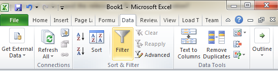
This will add a dropdown arrow on the first cell, click it, go to Text Filters, then Begins With. In the dialog type *PERFORMANCE*, and press OK. This will leave only the lines starting with *PERFORMANCE*, however, Excel will still show the original row numbers. Select the first column excluding the first line (by clicking on the 1st *PERFORMANCE* cell, then pressing Ctrl-Shift-Down Arrow), copy then paste the selected lines into a new sheet. This will reduce the number of displayed rows dramatically.
3. Split the text into columns using the Text-to-Columns feature
Tip: you can skip this step reduce the number of steps here, if you output your performance text comma-separated.
With the first column selected, in the Data pane, click Text to Columns. First, we’re going to split the string by *PERFORMANCE*, so select Fixed Width, then Next. Click and drag the arrow head one character to the right, then press Finish.

Now the first column only contains the word *PERFORMANCE*, so we can safely delete the entire first column.
Let’s repeat this step once more, this time selecting Delimited in the first page of the wizard, then Next. We want to split by the equals sign = so let’s type = into the text box next to Other. We can see in the preview how it will look like. Close the wizard by pressing Finish.

4. Adding the numbers together using PivotTables
Now that we have two columns, one containing the method name, and the other the time it took the method to execute, we can summarize it using a PivotTable. But first, we need to give the columns some meaning in the pivot table, so insert a new row before the fist row, and above the first column type Method, and above the second row type Time.

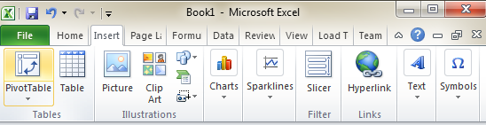
Select both columns except the first row (you can select just the two cells in row 2, then pressing Ctrl-Shift-Down Arrow). Go to Insert, then PivotTable, and press OK in the new dialog.
Drag the Time field down to where it says Values. This should create a field called Sum of Time. Drag the Method field into the Row Labels.

On the left we should now see all the methods with the time it took to run them nicely formatted:

And that’s it! We can now apply Excel’s sorting to the columns and perform other analytical data with our poor man’s performance profiling data.